Maxima Basics #3

Maxima Version 5.20.1
wxMaxima Version 0.8.4

(1)
The integrate() command is self-explanatory.

(%i1) integrate( log(x), x );

(%i2) integrate( log(x), x, 1, %e );

(%i3) f: x^2*sin(2*x);

(%i4) g: integrate( f, x );

(%i5) at( g, x=%pi ) - at( g, x=0 ); float(%);

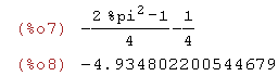
(%i7) integrate( f, x, 0, %pi ); float(%);

(%i9) kill( f, g );

(2)
The limit() command is self-explanatory. Use "inf" for infinity,
"minf" for negative infinity, "plus" for limits from the right, and
"minus" for limits from the left.

(%i10) limit( 3*sin(2*x)/(5*x), x, 0 );

(%i11) limit( cos(x)/x, x, inf );

(%i12) limit( sqrt(x^2+1)/x, x, minf );

(%i13) f: abs(x)/x;

(%i14) limit( f, x, 0, plus );

(%i15) limit( f, x, 0, minus );

(3)
Maxima can determine Taylor polynomials and series. The taylor() command is
self-explanatory. It's arguments are: expression, variable, center, order.
To convert the taylor() output to a polynomial, you can use taytorat() or ratsimp().

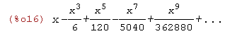
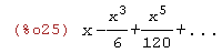
(%i16) taylor( sin(x), x, 0, 9 );

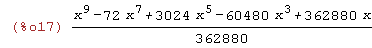
(%i17) taytorat(%);

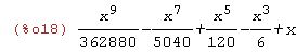
(%i18) expand(%);

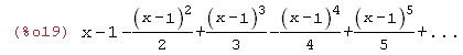
(%i19) taylor( log(x), x, 1, 5 );

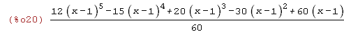
(%i20) taytorat(%);

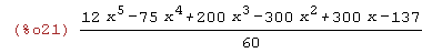
(%i21) ratsimp(%);

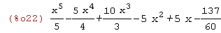
(%i22) expand(%);

(4)
To sketch graphs, you can use the Plot menu option. Choose the inline format
if you would like your graphs to appear on the worksheet itself.
Unfortunately, very few options are available from the Plot menu option.

(%i23) wxplot2d( [tan(x)], [x,-%pi/4,%pi/4] );

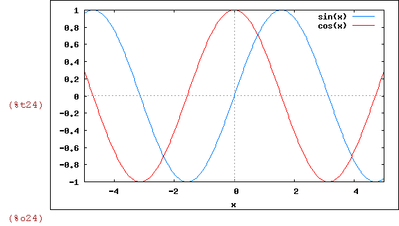
(%i24) wxplot2d( [sin(x), cos(x)], [x,-5,5] );

(%i25) f: taylor( sin(x), x, 0, 5 );

(%i26) plot2d( [sin(x), f], [x,-%pi,%pi] );

If everything worked correctly on your computer, the first two graphs above were inline
and the third graph was not. wxplot2d() will produce an inline graph. plot2d() will
produce a graph in a new window.

(5)
There are many plot options available if you load the "draw" package.
Here are some examples. You must close the graph window before returning
to the worksheet. You could put the graphs inline by using wxdraw2d()
instead of draw2d().

(%i27) load(draw)$

(%i28) draw2d( title = "sin(x) and its Maclaurin polynomials",
        xrange = [-4,4], yrange = [-2,2],
        xaxis = true, xaxis_type = solid, label(["x",3.75,-0.25]),
        yaxis = true, yaxis_type = solid, label(["y",0.25,1.75]),
        grid = true,
        color = black, line_width = 2, key = "sin(x)",
        explicit( sin(x), x, -%pi, %pi ),
        line_width = 1,
        color = blue, key = "P1(x)",
        explicit( taylor( sin(x), x, 0, 1 ), x, -%pi, %pi ),
        color = red, key = "P3(x)",
        explicit( taylor( sin(x), x, 0, 3 ), x, -%pi, %pi ),
        color = green, key = "P5(x)",
        explicit( taylor( sin(x), x, 0, 5 ), x, -%pi, %pi ) )$

(%i29) r(x):=sin(x)+3$
a: %pi$ b: 4*%pi$
draw3d(title = "Curve rotated about x-axis",
       enhanced3d=true, xu_grid=50, yv_grid=50,
       surface_hide=true,
       parametric_surface(u,r(u)*cos(v),r(u)*sin(v),
       u, a, b, v, 0, 2*%pi) )$

(%i33) draw2d( title = "Graphs of Implicit and Explicit Functions", yrange = [-4,4],
        xaxis = true, xaxis_type = solid, label(["x",3.75,-0.25]),
        yaxis = true, yaxis_type = solid, label(["y",0.25,3.75]),
        grid = true, nticks = 200, line_type = solid,
        key = "Implicit",
        implicit(y^2=x^3-2*x+1, x, -4,4, y, -4,4),
        color = red, nticks = 30, line_type = dots,
        key = "Explicit",
        explicit(x^2+1, x,-2,2) )$

(%i34) draw3d(enhanced3d = true, xu_grid=50, yv_grid=50,
       explicit(2^(-u^2 + v^2), u, -4, 4, v, -2, 2))$

(%i35) plot3d( x^2 - 3*sin(x)*y, [x, -5, 5], [y, -5, 5] )$